In aerospace engineering, linearized models are the cornerstone of control design. However, they are approximations. To truly understand the limits of an aircraft, you must look at the non-linear physics that take over when the “small perturbation” assumption fails.
During the Flight Dynamics (SAA0184) course at EESC-USP, the Zona de Turbulência group was tasked with a rigorous challenge: characterize the stability of a Cessna 182. Under the guidance of Prof. Ricardo Angélico, my role was to architect the computational environment, implementing the non-linear equations of motion to cross-validate our analytical predictions.
The Engineering Workflow
The project went beyond simple analysis. We needed to build a simulation environment capable of reproducing the aircraft’s dynamic behavior in the time domain.
1. Trimming the Aircraft
Before flying, you must find equilibrium. Leveraging the base scripts provided in the course, I adapted the Newton-Raphson routines to solve for the specific trim state ($V_{trim}, \alpha_{trim}, \delta_{e}, T$) of the Cessna 182. Using aerodynamic derivatives from Roskam (Appendix B), we defined the cruise condition at 5000ft:
\[CL_{trim} = \frac{mg}{\frac{1}{2} \rho U_{\infty}^2 S}\]2. Implementation: First Principles
The core of the simulation was built in Simulink using a “First Principles” approach. Instead of relying on black-box models, I constructed the longitudinal equations of motion in Body Axes, capturing the non-linear inertial coupling:
\[\begin{cases} \dot{u} = \frac{X}{m} - g \sin\theta - qw \\ \dot{w} = \frac{Z}{m} + g \cos\theta + qu \\ \dot{q} = \frac{M}{I_{yy}} \end{cases}\]These equations govern the accelerations, which are integrated to update the state vector $x = [u, w, q, \theta, x_e, z_e]^T$ at every time step.
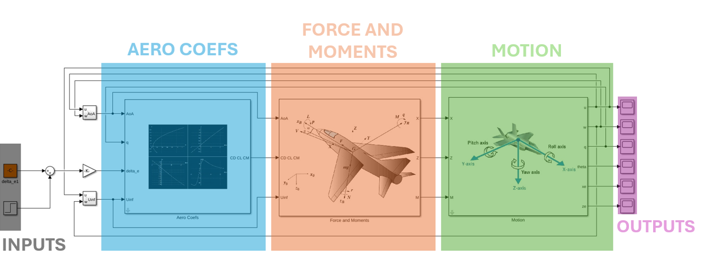 Figure 1: The Simulink environment I assembled to integrate the non-linear dynamics.
The Validation: Linear vs. Non-Linear
The “Eureka” moment came during the comparison phase. By linearizing the system into a State-Space representation ($\dot{x} = Ax + Bu$), we obtained the natural modes: the Short Period (fast, damped) and the Phugoid (slow, oscillatory).
When I injected a 1-degree elevator step into both models simultaneously:
- The Short Period response was nearly identical, proving the linear model is highly accurate for fast transients.
- The Phugoid started to show slight divergence over long time-scales, identifying exactly where non-linear gravity and drag couplings become relevant.
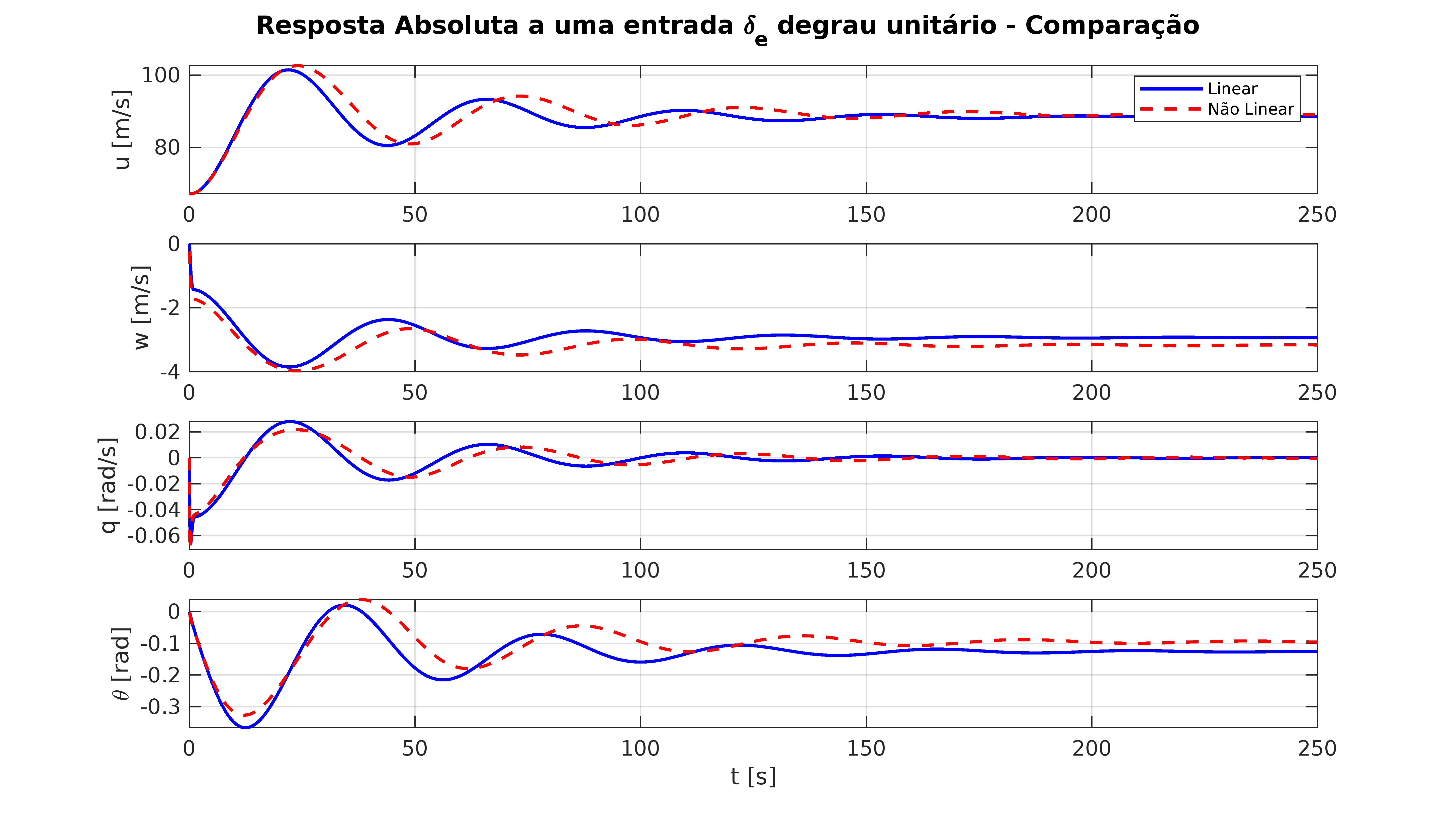 Figure 2: Validation results showing the non-linear simulation (Blue) tracking the linear prediction (Red).
Engineering Insight
This project reinforced a critical lesson in Model-Based Design: trust, but verify. By building the non-linear simulator from the ground up, we could mathematically validate the limitations of our linear control models. It was a practical exercise in understanding the trade-off between model complexity and computational cost.
Technical Assets
The complete implementation, including the adapted scripts and the Simulink model, is available here:
Discuss this Project
Are you interested in aircraft modeling or flight dynamics? Let’s discuss simulation architectures.